Introduction
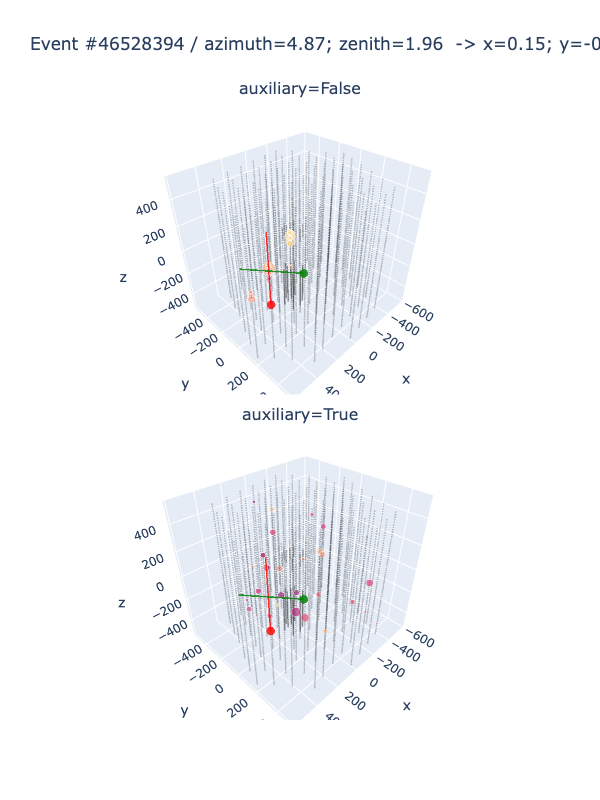
The IceCube Neutrino Observatory, located at the South Pole, is a cutting-edge research facility that is dedicated to studying high-energy neutrinos. Neutrinos are subatomic particles that are extremely difficult to detect because they interact very weakly with matter. However, they provide a unique window into the most energetic phenomena in the universe, such as supernovae, black holes, and gamma-ray bursts.One of the key challenges in studying neutrinos is determining their direction of arrival. To address this challenge, the IceCube detector uses a process called direction reconstruction. This involves detecting the charged particles produced by the interaction of the neutrino with the ice surrounding the detector and using this information to determine the direction of the neutrino.Recent developments in reconstruction algorithms have significantly improved the accuracy and precision of the direction reconstruction process. This has enabled researchers to identify the first high- energy neutrino source, a blazar, in 2018. Additionally, the addition of new detection modules to the IceCube detector has increased its sensitivity to lower energy neutrinos, expanding the range of neutrino sources that can be studied.
The reconstructed directions of neutrinos detected by IceCube have provided valuable insights into the high-energy universe. By studying the properties of these neutrinos, researchers can learn about the sources that produced them and the physical processes that govern their interactions.
This information can help us to better understand some of the most fundamental questions in astrophysics, such as the nature of dark matter and the origins of cosmic rays.In conclusion, the IceCube Neutrino Observatory is an essential tool for studying the most energetic phenomena in the universe. By improving the direction reconstruction process and expanding the capabilities of the detector, researchers will continue to make groundbreaking discoveries about the nature of the universe and its most extreme environments.
Google Colab Example:
You can embed your code snippets using Google Colab
Importing Libraries
In this project we are using PyTorch and Tensorflow as our ML and Deep Learning library for model building. Pandas and Numpy are used to parse and preprocess the parquet files.
    import numpy  as np

    import pandas  as pd

    import matplotlib.pyplot  as plt
Tip
Download the required data from here Link example
Extracting the datasets
Initially we read the parquet file from the local computer after installing and parse those parquet files and convert them into pandas dataframe. After that we preprocess the parquet file using pandas and numpy.
Importing Dataset :
    dataset = pd.read_csv('Data.csv')

    x = dataset.iloc[:,:-1].values

    y = dataset.iloc[:,-1].values
Pre-processing the dataset
IceCube neutrino detector processes vast amounts of raw data to identify the presence of neutrinos. The data pre-processing for IceCube involves several steps to reduce the data size, remove noise, and select the relevant events. The steps include calibration, filtering, hit reconstruction, pattern recognition, and event selection. Calibrating the detector sensors is necessary to ensure accurate data collection. Filtering helps to reduce noise and remove unwanted signals. Hit reconstruction involves identifying the location and time of each signal detected by the sensors. Pattern recognition algorithms group the hits into tracks or cascades, representing the possible trajectories of the neutrino interactions. Finally, event selection methods are applied to identify the events that are most likely to be neutrino interactions. The pre-processed data is then further analyzed to extract useful scientific information about neutrino properties and astrophysical phenomena.
Technologies used :
- Pandas
- Numpy
- Scikit-learn
- PyTorch
Code :
Preprocessing.py
  def prepare_sensors():
            sensors = pd.read_csv(INPUT_PATH / "sensor_geometry.csv").astype(
            {
            "sensor_id": np.int16, "x": np.float32,
            "y": np.float32,
            "z": np.float32,
            } )
            sensors["string"] = 0 sensors["qe"] = 1
            for i in range(len(sensors) // 60): start, end = i * 60, (i * 60) + 60 sensors.loc[start:end, "string"] = i
High Quantum Efficiency in the lower 50 DOMs
The "High Quantum Efficiency in the lower 50 DOMs" refers to an improvement in the sensitivity of the detector's lowermost 50 DOMs to detect Cherenkov radiation - the faint, bluish light emitted when neutrinos interact with the ice. This was achieved through the use of highly sensitive photomultiplier tubes and improved electronics in these DOMs, which allowed them to better distinguish the signal from background noise.
Preprocessing.py
  if i in range(78, 86):

            start_veto, end_veto = i * 60, (i * 60) + 10

            start_core, end_core = end_veto + 1, (i * 60) + 60

            sensors.loc[start_core:end_core, "qe"] = 1.35

            # Assume that "rde" (relative dom efficiency) is equivalent to QE

            sensors["x"] /= 500 sensors["y"] /= 500 sensors["z"] /= 500 sensors["qe"] -= 1.25 sensors["qe"] /= 0.25

            return sensors
Building GNN Model
To build a Graph Neural Network (GNN) model for the IceCube Neutrino detector, one would need to represent the detector as a graph. Each DOM (Digital Optical Module) can be considered as a node, and the adjacency matrix can be defined using the DOM locations and orientation. The input features can be the measured signals from each DOM. The GNN can then learn to extract the relevant features and predict the probability of neutrino detection based on the input signals. With the high quantum efficiency of the lower 50 DOMs, the GNN can potentially provide accurate detection of neutrinos in the detector.
  def calculate_distance_matrix (xyz_coords: Tensor) -> Tensor:
                diff = xyz_coords.unsqueeze(dim=2) - xyz_coords.T.unsqueeze(dim=0)
                return torch.sqrt(torch.sum(diff**2, dim=1))
class EuclideanGraphBuilder(nn.Module):

      def  init ( self,sigma: float,threshold: float = 0.0, columns: List[int] = None):

          # Check(s)

          if columns is None: columns = [0, 1, 2]
          # Base class constructor
          super(). init ()

          # Member variable(s) self._sigma = sigma self._threshold = threshold self._columns = columns

      def forward (self, data: Data) -> Data:

          # Constructs the adjacency matrix from the raw, DOM-level data and # returns this matrix

          xyz_coords = data.x[:, self._columns]

          # Construct block-diagonal matrix indicating whether pulses belong to
          # the same event in the batch

          batch_mask = data.batch.unsqueeze(dim=0) == data.batch.unsqueeze(dim=1)
          distance_matrix = calculate_distance_matrix(xyz_coords) affinity_matrix = torch.exp(-0.5 * distance_matrix**2 / self._sigma**2 )

          exp_row_sums = torch.exp(affinity_matrix).sum(axis=1) weighted_adj_matrix = torch.exp(affinity_matrix) / exp_row_sums.unsqueeze(dim=1)

          # Only include edges with weights that exceed the chosen threshold (and # are part of the same event)

          sources, targets = torch.where(
          (weighted_adj_matrix > self._threshold) & (batch_mask) )
          edge_weights = weighted_adj_matrix[sources, targets]
          data.edge_index = torch.stack((sources, targets)) data.edge_weight = edge_weights

          return  data
    class init (self, in_channels, out_channels=64, sigma=0.5 ):

                super(DenseDynBlock, self).init()

                self.GraphBuilder = EuclideanGraphBuilder(sigma=sigma)

                self.gnn = SAGEConv(in_channels, out_channels)
    class forward (self, data):

                data1 = self.GraphBuilder(data)

                x, edge_index, batch = data1.x, data1.edge_index, data1.batch x = self.gnn(x, edge_index)

                data1.x = torch.cat((x, data.x), 1)

                return data1
MODEL: GRAPH NEURAL NETWORK
    def forward(self, data):

                    x, edge_index, batch = data.x, data.edge_index, data.batch data.x = self.head(x, edge_index)
                    feats = [data.x]
                    for i in range(self.n_blocks-1):
                        data = self.gnn[i](data)
                        feats.append(data.x)
                        feats = torch.cat(feats, 1)
                        x = pyg_nn.global_mean_pool(feats, data.batch) out = F.relu(self.linear(x))

                    return out
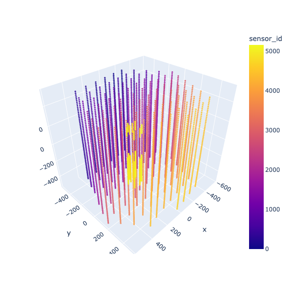
Neutrino Angles Prediction
    geometry = pd.read_csv("D:/Neutrinos/sensor_geometry.csv")

    import plotly.express as px

    fig = px.scatter_3d(geometry, x='x', y='y', z='z', opacity=0.8, color='sensor_id')
    fig.update_traces(marker_size = 2)
    fig.update_layout(height = 600, width=600)
    fig.show()
This is the sample visualised data